How-to guides
This section contains goal-oriented guides on the features of scikit-fem.
Finding degrees-of-freedom
Often the goal is to constrain DOFs on a specific part of
the boundary. The DOF numbers have one-to-one correspondence with
the rows and the columns of the finite element system matrix,
and the DOFs are typically passed to functions
such as condense() or enforce()
that modify the linear system to implement the boundary conditions.
Currently the main tool for finding DOFs is
get_dofs().
Let us look at the use of this method through an example
with a triangular mesh
and the quadratic Lagrange element:
>>> from skfem import MeshTri, Basis, ElementTriP2
>>> m = MeshTri().refined(2).with_defaults()
>>> basis = Basis(m, ElementTriP2())
Normally, a list of facet indices is provided
for get_dofs()
and it will find the matching DOF indices.
However, for convenience,
we can provide an indicator function to
get_dofs() and it will find the
DOFs on the matching facets (via their midpoints):
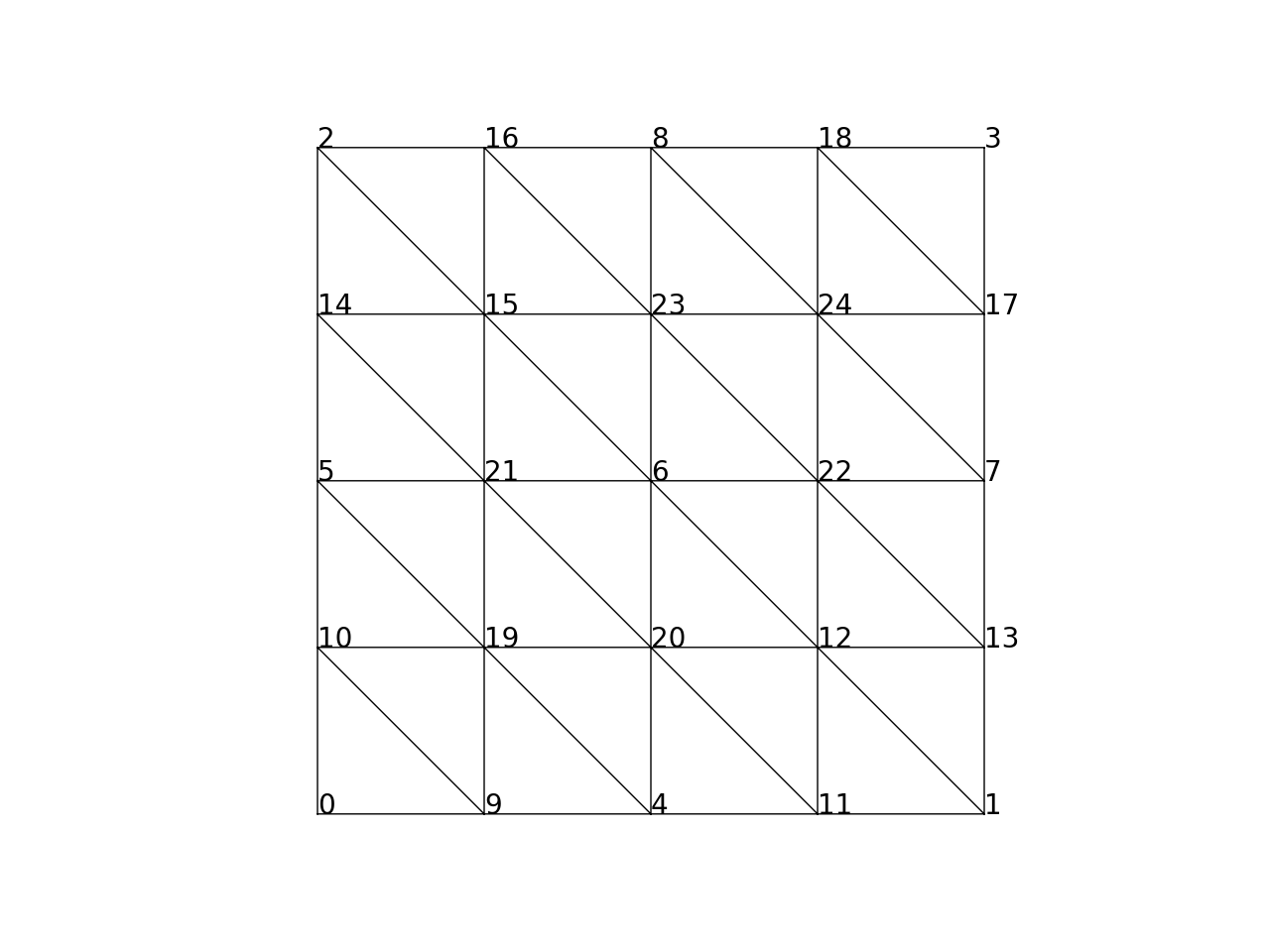
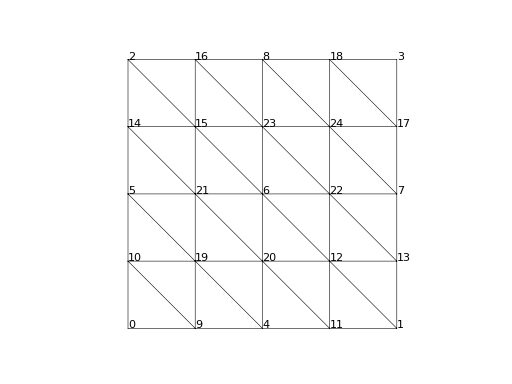
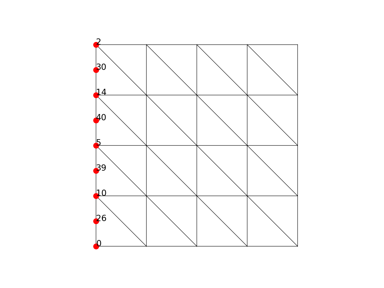
>>> dofs = basis.get_dofs(lambda x: x[0] == 0.)
>>> dofs.nodal
{'u': array([ 0,  2,  5, 10, 14], dtype=int32)}
>>> dofs.facet
{'u': array([26, 30, 39, 40], dtype=int32)}
Here is a visualization of the nodal DOFs:
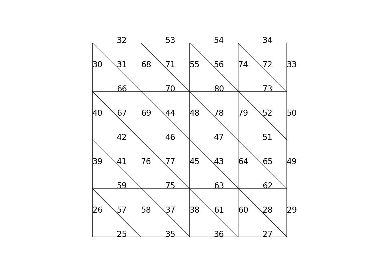
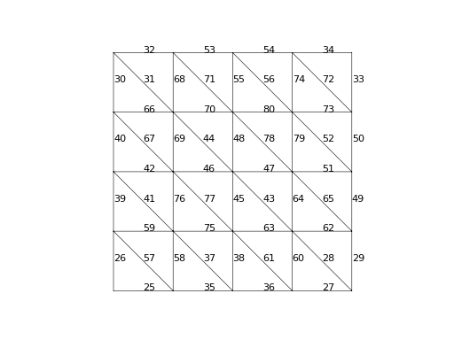
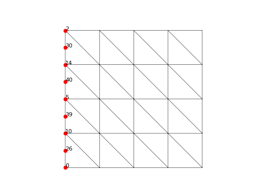
This quadratic Lagrange element has one DOF per node and one DOF per facet. Globally, the facets have their own numbering scheme starting from zero, while the corresponding DOFs are offset by the total number of nodal DOFs:
>>> dofs.facet['u']
array([26, 30, 39, 40], dtype=int32)
Here is a visualization of the facet DOFs:
The keys in the above dictionaries indicate the type of the DOF according to the following table:
Key |
Description |
|---|---|
|
Point value |
|
Normal derivative |
|
Partial derivative w.r.t. \(x\) |
|
Second partial derivative w.r.t \(x\) |
|
Normal component of a vector field (e.g., Raviart-Thomas) |
|
Tangential component of a vector field (e.g., Nédélec) |
|
First component of a vector field |
|
Partial derivative of the first component w.r.t. \(x\) |
|
First component of the first component in a composite field |
|
Description not available (e.g., hierarchical or bubble DOFs) |
Most of the time we just want an array of all DOFs with the key u.
This can be obtained as follows:
>>> dofs.all(['u'])
array([ 0,  2,  5, 10, 14, 26, 30, 39, 40], dtype=int32)
>>> dofs.flatten()  # all DOFs, no matter which key
array([ 0,  2,  5, 10, 14, 26, 30, 39, 40], dtype=int32)
If a set of facets is tagged, the name of the tag can be passed
also to get_dofs():
>>> dofs = basis.get_dofs('left')
>>> dofs.flatten()
array([ 0,  2,  5, 10, 14, 26, 30, 39, 40], dtype=int32)
Many DOF types have a well-defined location. These DOF locations can be found as follows:
>>> basis.doflocs[:, dofs.flatten()]
array([[0.   , 0.   , 0.   , 0.   , 0.   , 0.   , 0.   , 0.   , 0.   ],
       [0.   , 1.   , 0.5  , 0.25 , 0.75 , 0.125, 0.875, 0.375, 0.625]])
See Indexing of the degrees-of-freedom for more details.
Performing projections
A common issue in finite element analysis is that you have either an analytical function with a given expression or a finite element function defined on one basis, while what you would like to have instead is the same function defined on another finite element basis.
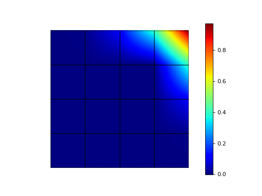
We can use \(L^2\) projection to find discrete counterparts of functions or transform from one finite element basis to another. For example, suppose we have \(u_0(x,y) = x^3 y^3\) defined on the boundary of the domain and want to find the corresponding discrete function which is extended by zero in the interior of the domain. Technically, you could explicitly assemble and solve the linear system corresponding to: find \(\widetilde{u_0} \in V_h\) satisfying
However, this is so common that we have a shortcut command
project():
>>> import numpy as np
>>> from skfem import *
>>> m = MeshQuad().refined(2)
>>> basis = FacetBasis(m, ElementQuad1())
>>> u0 = lambda x: x[0] ** 3 * x[1] ** 3
>>> u0t = basis.project(u0)
>>> np.abs(np.round(u0t, 5))
array([1.0000e-05, 8.9000e-04, 9.7054e-01, 8.9000e-04, 6.0000e-05,
       6.0000e-05, 1.0944e-01, 1.0944e-01, 0.0000e+00, 2.0000e-05,
       2.0000e-05, 2.4000e-04, 8.0200e-03, 3.9797e-01, 3.9797e-01,
       2.4000e-04, 8.0200e-03, 0.0000e+00, 0.0000e+00, 0.0000e+00,
       0.0000e+00, 0.0000e+00, 0.0000e+00, 0.0000e+00, 0.0000e+00])

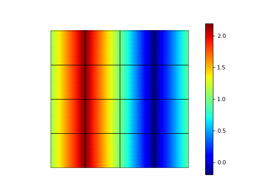
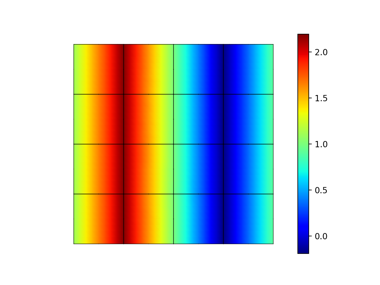
As another example, we can also project over the entire domain:
>>> basis = Basis(m, ElementQuad1())
>>> f = lambda x: np.sin(2. * np.pi * x[0]) + 1.
>>> fh = basis.project(f)
>>> np.abs(np.round(fh, 5))
array([1.09848, 0.90152, 0.90152, 1.09848, 1.     , 1.09848, 0.90152,
       1.     , 1.     , 2.19118, 1.09848, 0.19118, 0.90152, 0.90152,
       0.19118, 1.09848, 2.19118, 1.     , 2.19118, 0.19118, 1.     ,
       2.19118, 0.19118, 0.19118, 2.19118])

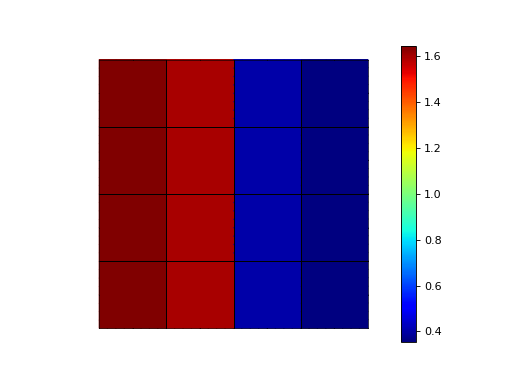
Or alternatively, we can use the same command to project from one finite element basis to another:
>>> basis0 = basis.with_element(ElementQuad0())
>>> fh = basis0.project(basis.interpolate(fh))
>>> np.abs(np.round(fh, 5))
array([1.64483, 0.40441, 0.40441, 1.64483, 1.59559, 0.35517, 0.35517,
       1.59559, 1.59559, 0.35517, 0.35517, 1.59559, 1.64483, 0.40441,
       0.40441, 1.64483])
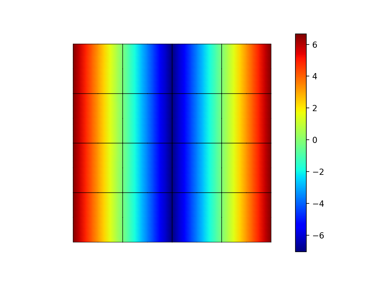
We can also interpolate the gradient at quadrature points and then project:
>>> f = lambda x: np.sin(2. * np.pi * x[0]) + 1.
>>> fh = basis.project(f)  # P1
>>> fh = basis.project(basis.interpolate(fh).grad[0])  # df/dx
>>> np.abs(np.round(fh, 5))
array([6.6547 , 6.6547 , 6.6547 , 6.6547 , 7.04862, 6.6547 , 6.6547 ,
       7.04862, 7.04862, 0.19696, 6.6547 , 0.19696, 6.6547 , 6.6547 ,
       0.19696, 6.6547 , 0.19696, 7.04862, 0.19696, 0.19696, 7.04862,
       0.19696, 0.19696, 0.19696, 0.19696])

Discrete functions in the forms
It is a common pattern to reuse an existing finite element function in the forms.
Everything within the form is expressed at the quadrature points and
the finite element functions must be interpolated
from nodes to the
quadrature points through interpolate().
For example, consider a fixed-point iteration for the nonlinear problem
We can repeatedly find \(u_{k+1} \in H^1_0(\Omega)\) which satisfies
The bilinear form depends on the previous solution \(u_k\) which can be defined as follows:
>>> import skfem as fem
>>> from skfem.models.poisson import unit_load
>>> from skfem.helpers import grad, dot
>>> @fem.BilinearForm
... def bilinf(u, v, w):
...     return (w.u_k + .1) * dot(grad(u), grad(v))
The previous solution \(u_k\) is interpolated at quadrature points using
interpolate() and then provided to
assemble() as a keyword argument:
>>> m = fem.MeshTri().refined(3)
>>> basis = fem.Basis(m, fem.ElementTriP1())
>>> b = unit_load.assemble(basis)
>>> x = 0. * b.copy()
>>> for itr in range(20):  # fixed point iteration
...     A = bilinf.assemble(basis, u_k=basis.interpolate(x))
...     x = fem.solve(*fem.condense(A, b, I=m.interior_nodes()))
...     print(round(x.max(), 10))
0.7278262868
0.1956340215
0.3527261363
0.2745541843
0.3065381711
0.2921831118
0.298384264
0.2956587119
0.2968478347
0.2963273314
0.2965548428
0.2964553357
0.2964988455
0.2964798184
0.2964881386
0.2964845003
0.2964860913
0.2964853955
0.2964856998
0.2964855667
Note
Inside the form definition, w is a dictionary of user provided
arguments and additional default keys. By default, w['x'] (accessible
also as w.x) corresponds to the global coordinates and w['h']
(accessible also as w.h) corresponds to the local mesh parameter.
Postprocessing the solution
After solving the finite element system \(Ax=b\), it is common to calculate derived quantities. The most common techniques are:
Calculating gradient fields using the technique described at the end of Performing projections.
Using
Functionalwrapper to calculate integrals over the finite element solution.
The latter consists of writing the integrand as a function
and decorating it using Functional.
This is similar to the use of BilinearForm
and LinearForm wrappers
expect that the function wrapped by Functional
should accept only a single argument w.
The parameter w is a dictionary containing all the default keys
(e.g., w['h'] for mesh parameter and w['x'] for global
coordinates) and any user provided arguments that can
be arbitrary finite element functions interpolated at the quadrature points
using interpolate().
As a simple example, we calculate the integral of the finite element
solution to the Poisson problem with a unit load:
>>> from skfem import *
>>> from skfem.models.poisson import laplace, unit_load
>>> mesh = MeshTri().refined(2).with_defaults()
>>> basis = Basis(mesh, ElementTriP2())
>>> A = laplace.assemble(basis)
>>> b = unit_load.assemble(basis)
>>> x = solve(*condense(A, b, D=basis.get_dofs('left')))
>>> @Functional
... def integral(w):
...    return w['uh']  # grad, dot, etc. can be used here
>>> float(round(integral.assemble(basis, uh=basis.interpolate(x)), 5))
0.33333

Similarly we can calculate the integral of its derivative:
>>> @Functional
... def diffintegral(w):
...    return w['uh'].grad[0]  # derivative wrt x
>>> float(round(diffintegral.assemble(basis, uh=basis.interpolate(x)), 5))
0.5
We can also calculate integrals over (a subset of) the boundary
using FacetBasis:
>>> fbasis = basis.boundary('left')
>>> @Functional
... def bndintegral(w):
...    return w['uh'].grad[1]  # derivative wrt y
>>> float(round(bndintegral.assemble(fbasis, uh=fbasis.interpolate(x)), 5))
0.0
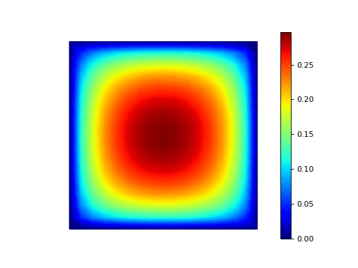
Visualizing the solution
After solving the finite element system \(Ax=b\), it is common to visualize the solution or other derived fields. The library includes some basic 2D visualization routines implemented using matplotlib. For more complex visualizations, we suggest that the solution is saved to VTK and a visualization is created using Paraview.
The main routine for creating 2D visualizations using matplotlib is
skfem.visuals.matplotlib.plot() and it accepts the basis
object and the solution vector as its arguments:
>>> from skfem import *
>>> from skfem.models.poisson import laplace, unit_load
>>> mesh = MeshTri().refined(2)
>>> basis = Basis(mesh, ElementTriP2())
>>> A = laplace.assemble(basis)
>>> b = unit_load.assemble(basis)
>>> x = solve(*condense(A, b, D=basis.get_dofs()))
>>> from skfem.visuals.matplotlib import plot
>>> plot(basis, x)
<Axes: >

It accepts various optional arguments to make the plots nicer, some of which have been demonstrated in Gallery of examples. For example, here is the same solution as above with different settings:
>>> plot(basis, x, shading='gouraud', colorbar={'orientation': 'horizontal'}, nrefs=3)
<Axes: >

The routine is based on matplotlib.pyplot.tripcolor command and shares
its limitations.
For more control we suggest that the solution is saved to a VTK file for
visualization in Paraview. Saving of the solution is done through the
mesh object method skfem.mesh.Mesh.save()
and it requires giving an array with one value per node of the mesh.
In order to properly visualize other than piecewise linear finite element bases, the mesh must be refined and the solution interpolated for visualization only:
>>> rmesh, rx = basis.refinterp(x, nrefs=3)  # refine and interpolate
>>> rmesh.save('sol.vtk', point_data={'x': rx})
Another option to visualize high order finite element functions
would be to first project the solution
onto a piecewise linear finite element basis
as described in Performing projections.
Piecewise linear finite element solutions can be passed directly
to point_data keyword argument of skfem.mesh.Mesh.save().
Please see Gallery of examples for more examples of visualization.