Gallery of examples
This page contains an overview of the examples contained in the source code repository.
Poisson equation
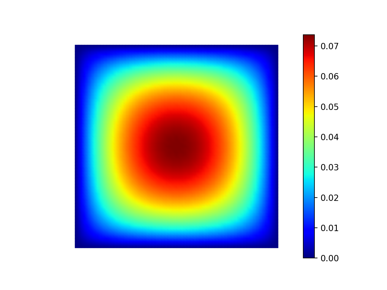
Example 1: Poisson equation with unit load
This example solves the Poisson problem \(-\Delta u = 1\) with the Dirichlet boundary condition \(u = 0\) in the unit square using piecewise-linear triangular elements.

The solution of Example 1.
See the source code of example 01 for more information.
Example 7: Discontinuous Galerkin method
This example solves the Poisson problem \(-\Delta u = 1\) with \(u=0\) on the boundary using discontinuous Galerkin method. The finite element basis is piecewise-quartic but discontinuous over the element edges.

The solution of Example 7.
See the source code of example 07 for more information.
Example 12: Postprocessing
This example demonstrates postprocessing the value of a functional, Boussinesq’s k-factor.
The solution of Example 12.
See the source code of example 12 for more information.
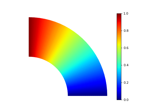
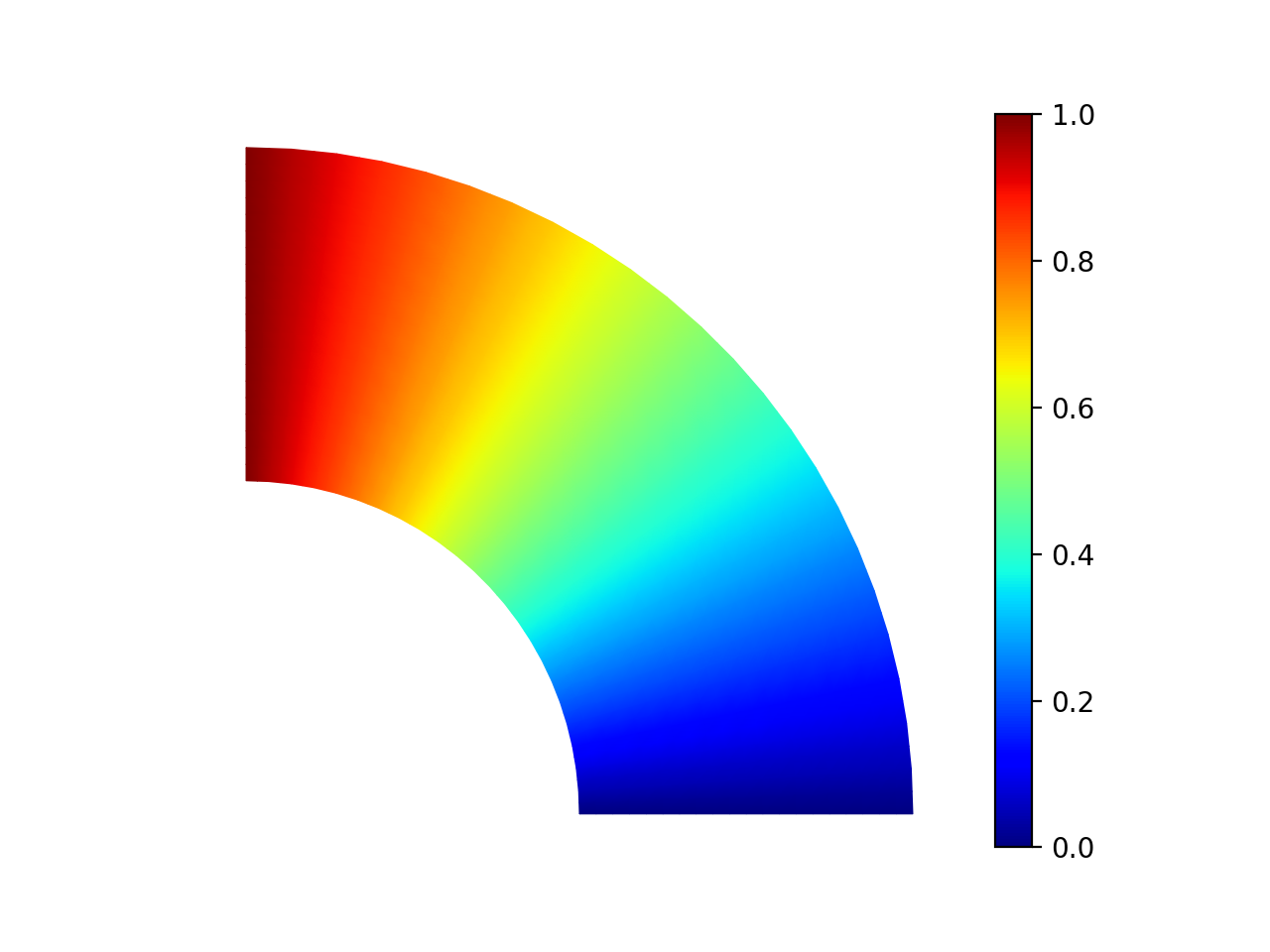
Example 13: Laplace with mixed boundary conditions
This example solves \(\Delta u = 0\) in \(\Omega=\{(x,y):1<x^2+y^2<4,~0<\theta<\pi/2\}\), where \(\tan \theta = y/x\), with \(u = 0\) on \(y = 0\), \(u = 1\) on \(x = 0\), and \(\frac{\partial u}{\partial n} = 0\) on the rest of the boundary.

The solution of Example 13.
See the source code of example 13 for more information.
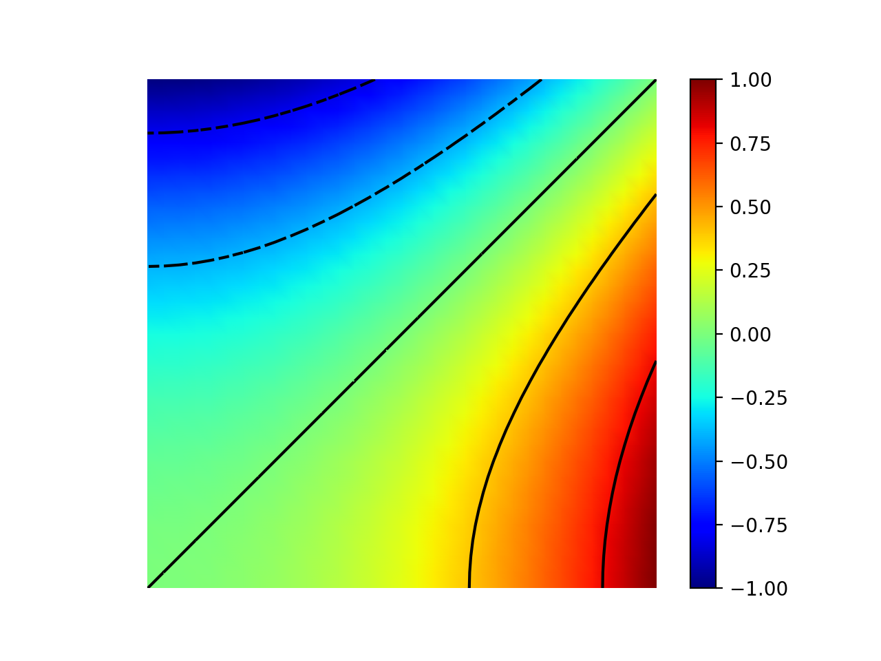
Example 14: Laplace with inhomogeneous boundary conditions
This example demonstrates how to impose coordinate-dependent Dirichlet conditions for the Laplace equation \(\Delta u = 0\). The solution will satisfy \(u=x^2 - y^2\) on the boundary of the square domain.

The solution of Example 14.
See the source code of example 14 for more information.
Example 15: One-dimensional Poisson equation
This example solves \(-u'' = 1\) in \((0,1)\) with the boundary condition \(u(0)=u(1)=0\).

The solution of Example 15.
See the source code of example 15 for more information.
Example 9: Three-dimensional Poisson equation
This example solves \(-\Delta u = 1\) with \(u=0\) on the boundary using linear tetrahedral elements and a preconditioned conjugate gradient method.

The solution of Example 9 on a cross-section of the tetrahedral mesh. The figure was created using ParaView.
See the source code of example 09 for more information.
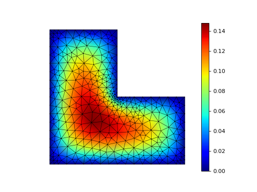
Example 22: Adaptive Poisson equation
This example solves Example 1 adaptively in an L-shaped domain. Using linear elements, the error indicators read \(\eta_K^2 = h_K^2 \|f\|_{0,K}^2\) and \(\eta_E^2 = h_E \| [[\nabla u_h \cdot n ]] \|_{0,E}^2\) for each element \(K\) and edge \(E\).

The final solution of Example 22.
See the source code of example 22 for more information.
Example 37: Mixed Poisson equation
This example solves the mixed formulation of the Poisson equation using the lowest order Raviart-Thomas elements.

The piecewise constant solution field. The figure was created using ParaView.
See the source code of example 37 for more information.
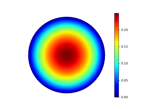
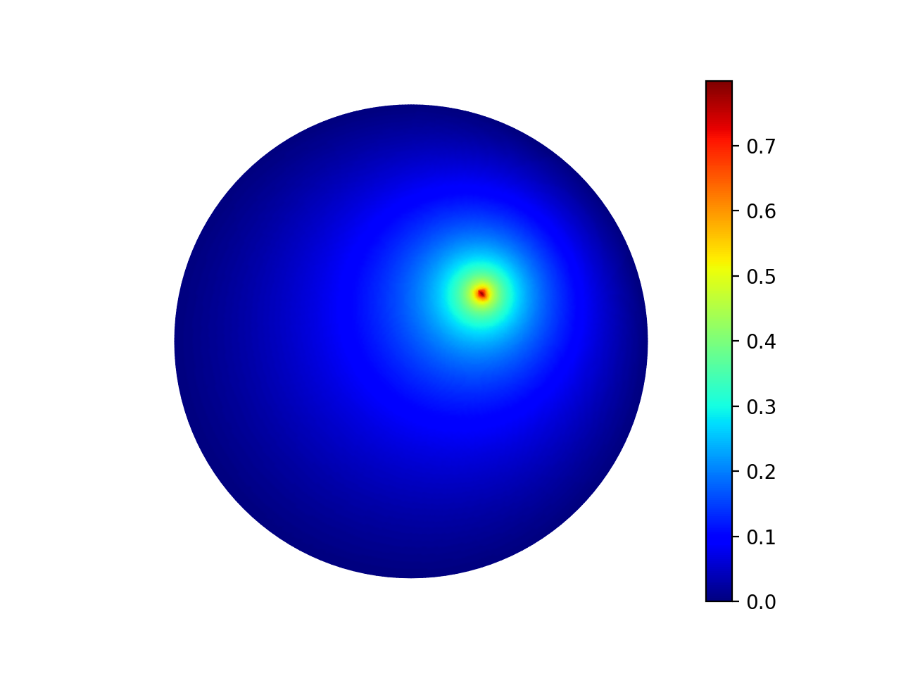
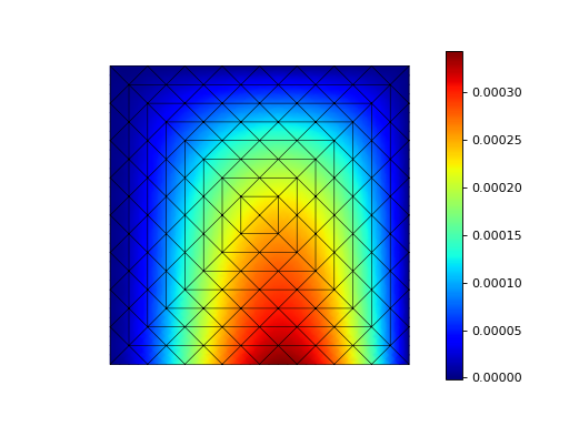
Example 38: Point source
Point sources require different assembly to other linear forms.
This example computes the Green’s function for a disk; i.e. the solution of the Dirichlet problem for the Poisson equation with the source term concentrated at a single interior point \(\boldsymbol{s}\), \(-\Delta u = \delta (\boldsymbol{x} - \boldsymbol{s})\).
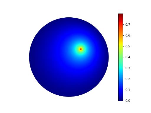
The scalar potential in the disk with point source at (0.3, 0.2).
See the source code of example 38 for more information.
Example 40: Hybridizable discontinuous Galerkin method
This examples solves the Poisson equation with unit load using a technique where the finite element basis is first discontinous across element edges and then the continuity is recovered with the help of Lagrange multipliers defined on the mesh skeleton (i.e. a “skeleton mesh” consisting only of the edges of the original mesh).
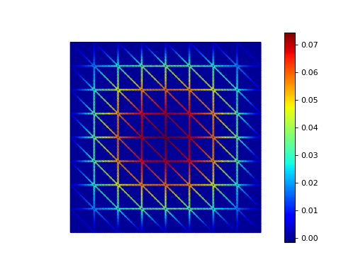
The solution of Example 40 on the skeleton mesh.
See the source code of example 40 for more information.
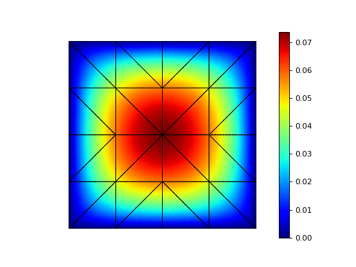
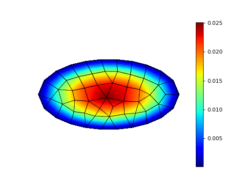
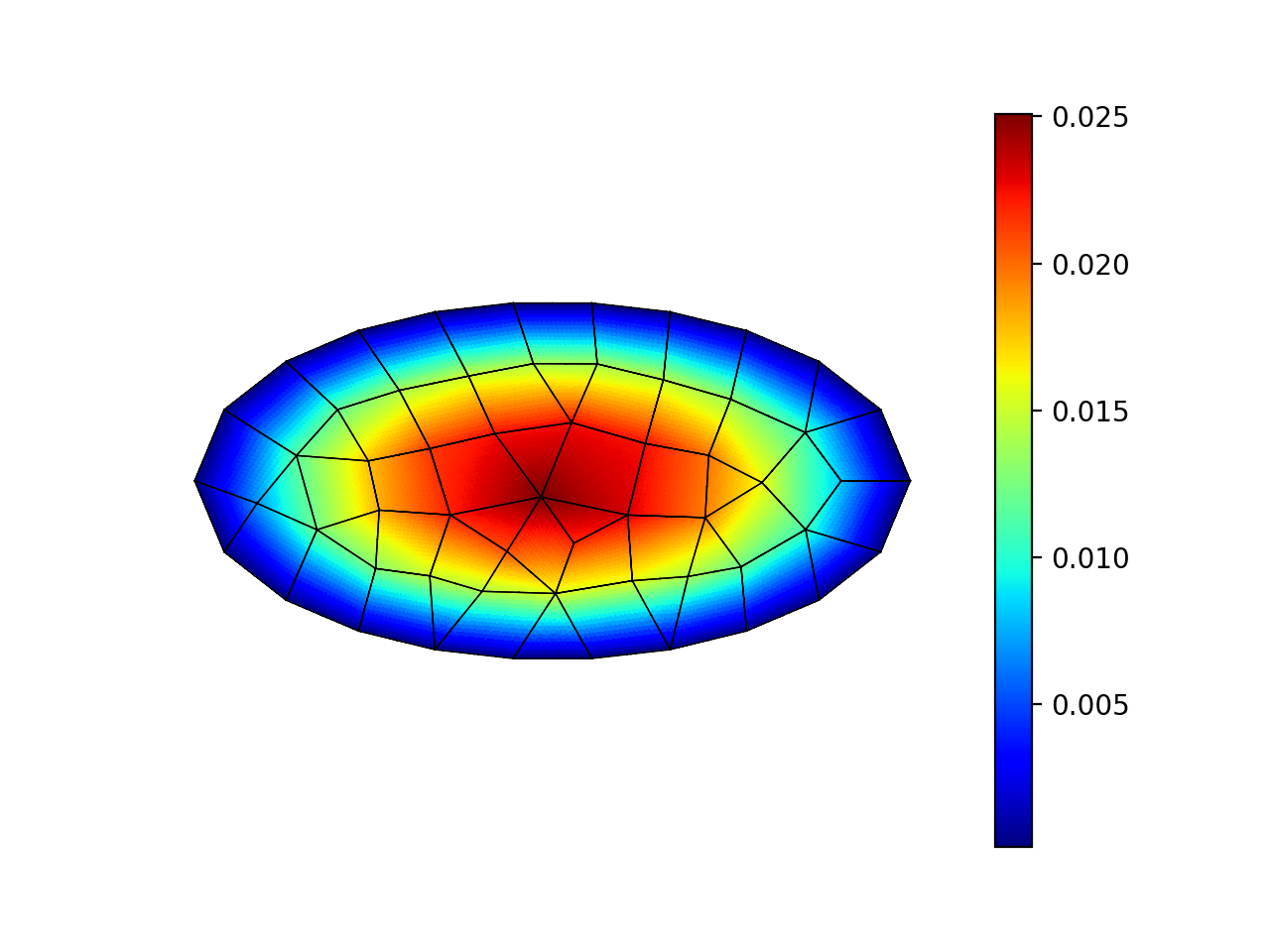
Example 41: Mixed meshes
This example solves the Poisson equation with unit load on a mesh consisting of both triangles and quadrilaterals. The support for mixed meshes is preliminary and works only for elements with nodal or internal degrees-of-freedom (sharing face and edge DOFs between mesh types is work-in-progress).

The solution of Example 41 on the mesh with both triangles and quadrilaterals.
See the source code of example 41 for more information.
Solid mechanics
Example 2: Kirchhoff plate bending problem
This example solves the biharmonic Kirchhoff plate bending problem \(D \Delta^2 u = f\) in the unit square with a constant loading \(f\), bending stiffness \(D\) and a combination of clamped, simply supported and free boundary conditions.

The solution of Example 2.
See the source code of example 02 for more information.
Example 3: Linear elastic eigenvalue problem
This example solves the linear elastic eigenvalue problem \(\mathrm{div}\,\sigma(u)= \lambda u\) with the displacement fixed on the left boundary.

The fifth eigenmode of Example 3.
See the source code of example 03 for more information.
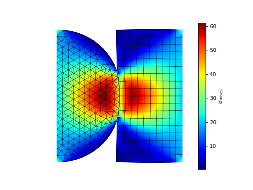
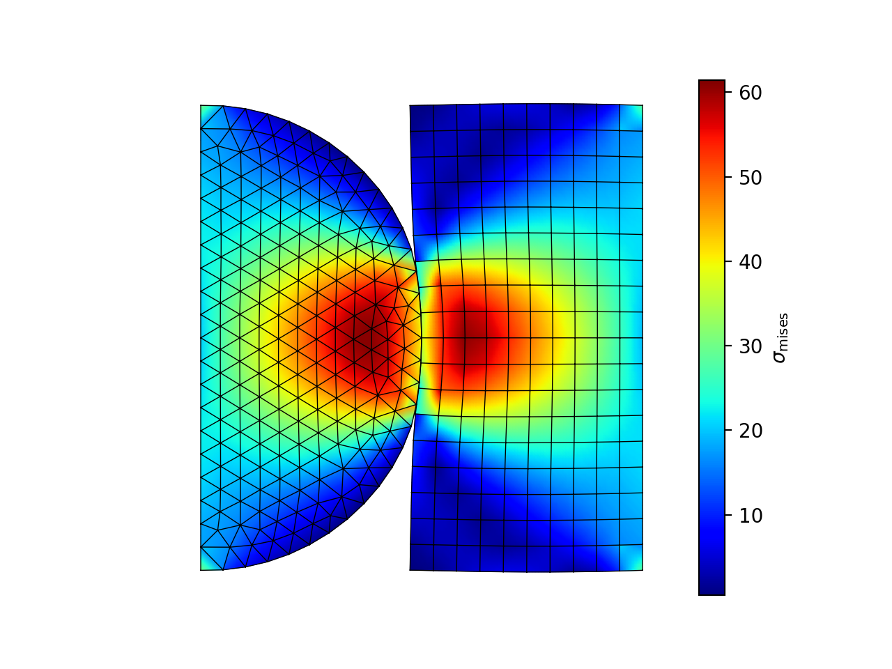
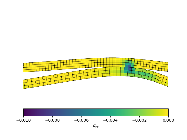
Example 4: Linearized contact problem
This example solves a single interation of the contact problem between two elastic bodies using the Nitsche’s method. Triangular and quadrilateral second-order elements are used in the discretization of the two elastic bodies.

The displaced meshes and the von Mises stress of Example 4.
See the source code of example 04 for more information.
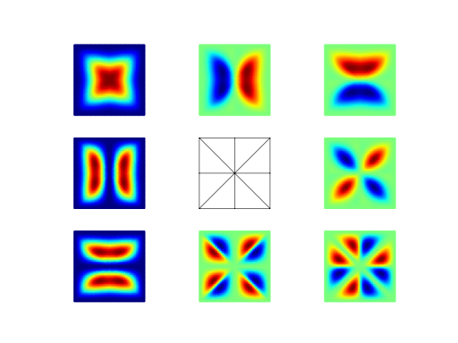
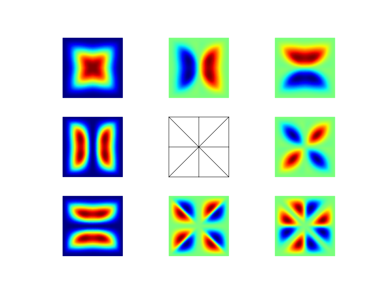
Example 8: Argyris basis functions
This example visualizes the \(C^1\)-continuous fifth degree Argyris basis functions on a simple triangular mesh. This element can be used in the conforming discretization of biharmonic problems.

The Argyris basis functions of Example 8 corresponding to the middle node and the edges connected to it.
See the source code of example 08 for more information.
Example 11: Three-dimensional linear elasticity
This example solves the three-dimensional linear elasticity equations \(\mathrm{div}\,\sigma(u)=0\) using trilinear hexahedral elements. Dirichlet conditions are set on the opposing faces of a cube: one face remains fixed and the other is displaced slightly outwards.

The displaced mesh of Example 11. The figure was created using ParaView.
See the source code of example 11 for more information.
Example 21: Structural vibration
This example demonstrates the solution of a three-dimensional vector-valued eigenvalue problem by considering the vibration of an elastic structure.

The first eigenmode of Example 21.
See the source code of example 21 for more information.
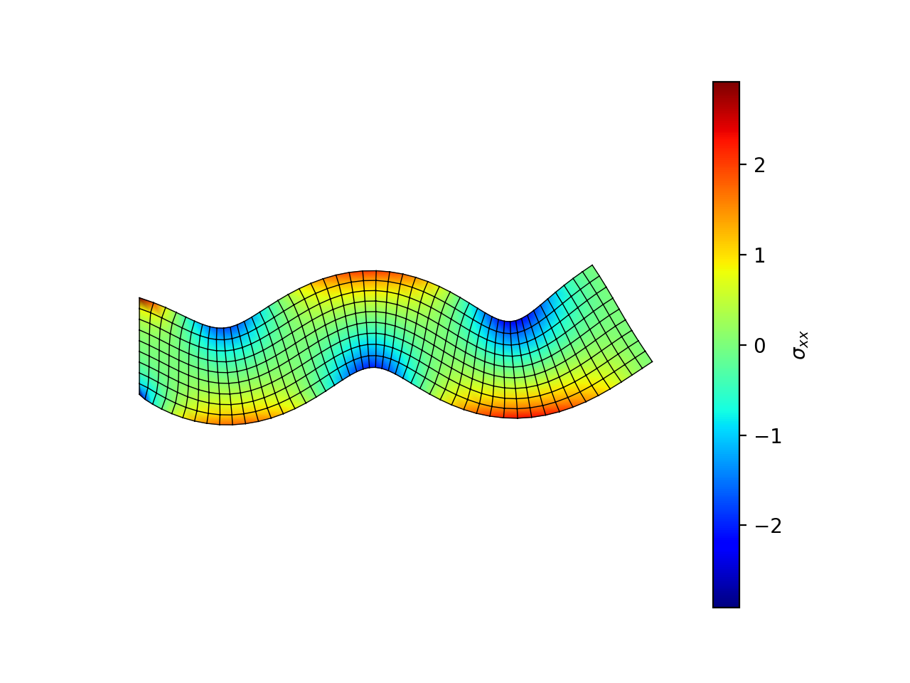
Example 34: Euler-Bernoulli beam
This example solves the Euler-Bernoulli beam equation \((EI u'')'' = 1\) with the boundary conditions \(u(0)=u'(0) = 0\) and using cubic Hermite elements. The exact solution at \(x=1\) is \(u(1)=1/8\).

The solution of Example 34.
See the source code of example 34 for more information.
Example 36: Nearly incompressible hyperelasticity
This example demonstrates the implementation of a two field mixed formulation for nearly incompressible Neo-Hookean solids.

The displacement contour of Example 36. The figure was created using ParaView.
See the source code of example 36 for more information.
Example 43: Hyperelasticity - Total Lagrangian formulation
This example demonstrates Newton’s method applied to the classical formulation of a hyperelastic Neo-Hookean solid using the Total Lagrangian formulation.

The deformed mesh of Example 43. The figure was created using vedo.
See the source code of example 43 for more information.
Example 55: Hyperelasticity - Updated Lagrangian formulation
This example demonstrates Newton’s method applied to the classical formulation of a hyperelastic Neo-Hookean solid using the Updated Lagrangian formulation where the weak form and derivatives therein are evaluated w.r.t. the current configuration. The non-linearity of the material model relies on the deformatoin gradient which needs the spatial derivatives w.r.t. the reference configuration. To that end we use two meshes whereas one is updated in every iteration to provide the spatial deriavtives w.r.t. the current configuration and the other mesh is used to provide the derivatives w.r.t. to the reference configuration.
The deformed mesh of Example 55 matches the one of example 43 exactly. The figure was created using vedo.
See the source code of example 55 for more information.
Example 51: Contact problem
This example solves the so-called large deformation contact problem between two nonlinear elastic solids.
The deformed mesh and stress of Example 51.
See the source code of example 51 for more information.
Fluid mechanics
Example 18: Stokes equations
This example solves for the creeping flow problem in the primitive variables, i.e. velocity and pressure instead of the stream-function. These are governed by the Stokes momentum \(- \nu\Delta\boldsymbol{u} + \rho^{-1}\nabla p = \boldsymbol{f}\) and the continuity equation \(\nabla\cdot\boldsymbol{u} = 0\).

The streamlines of Example 18.
See the source code of example 18 for more information.
Example 20: Creeping flow via stream-function
This example solves the creeping flow problem via the stream-function formulation. The stream-function \(\psi\) for two-dimensional creeping flow is governed by the biharmonic equation \(\nu \Delta^2\psi = \mathrm{rot}\,\boldsymbol{f}\) where \(\nu\) is the kinematic viscosity (assumed constant), \(\boldsymbol{f}\) the volumetric body-force, and \(\mathrm{rot}\,\boldsymbol{f} = \partial f_y/\partial x - \partial f_x/\partial y\). The boundary conditions at a wall are that \(\psi\) is constant (the wall is impermeable) and that the normal component of its gradient vanishes (no slip)

The velocity field of Example 20.
See the source code of example 20 for more information.
Example 24: Stokes flow with inhomogeneous boundary conditions
This example solves the Stokes flow over a backward-facing step with a parabolic velocity profile at the inlet.

The streamlines of Example 24.
See the source code of example 24 for more information.
Example 29: Linear hydrodynamic stability
The linear stability of one-dimensional solutions of the Navier-Stokes equations is governed by the Orr-Sommerfeld equation. This is expressed in terms of the stream-function \(\phi\) of the perturbation, giving a two-point boundary value problem \(\alpha\phi(\pm 1) = \phi'(\pm 1) = 0\) for a complex fourth-order ordinary differential equation,
where \(U(z)\) is the base velocity profile, \(c\) and \(\alpha\) are the wavespeed and wavenumber of the disturbance, and \(R\) is the Reynolds number.

The results of Example 29.
See the source code of example 29 for more information.
Example 30: Krylov-Uzawa method for the Stokes equation
This example solves the Stokes equation iteratively in a square domain.

The pressure field of Example 30.
See the source code of example 30 for more information.
Example 32: Block diagonally preconditioned Stokes solver
This example solves the Stokes problem in three dimensions, with an algorithm that scales to reasonably fine meshes (a million tetrahedra in a few minutes).

The velocity and pressure fields of Example 32, clipped in the plane of spanwise symmetry, z = 0. The figure was created using ParaView 5.8.1.
See the source code of example 32 for more information.
Example 42: Periodic meshes
This example solves the advection equation on a periodic square mesh.

The solution of Example 42 on a periodic mesh.
See the source code of example 42 for more information.
Example 50: Advection-diffusion in non-uniform flow
This example solves the advection-diffusion problem for the temperature distribution around a cold sphere in a warm liquid. The liquid flow is modeled using the Stokes flow field. The thermal diffusivity to advection ratio is controlled by the Peclet number. The problem is solved in a cylindrical coordinate system (hence a different definition of the Laplacian).
Temperature distribution of Example 50. Liquid behind the sphere is colder than the incoming one.
See the source code of example 50 for more information.
Heat transfer
Example 17: Insulated wire
This example solves the steady heat conduction with generation in an insulated wire. In radial coordinates, the governing equations read: find \(T\) satisfying \(\nabla \cdot (k_0 \nabla T) + A = 0,~0<r<a\), and \(\nabla \cdot (k_1 \nabla T) = 0,~a<r<b\), with the boundary condition \(k_1 \frac{\partial T}{\partial r} + h T = 0\) on \(r=b\).

The solution of Example 17.
See the source code of example 17 for more information.
Example 19: Heat equation
This example solves the heat equation \(\frac{\partial T}{\partial t} = \kappa\Delta T\) in the domain \(|x|<w_0\) and \(|y|<w_1\) with the initial value \(T_0(x,y) = \cos\frac{\pi x}{2w_0}\cos\frac{\pi y}{2w_1}\) using the generalized trapezoidal rule (“theta method”) and fast time-stepping by factorizing the evolution matrix once and for all.

The solution of Example 19.
See the source code of example 19 for more information.
Example 25: Forced convection
This example solves the plane Graetz problem with the governing advection-diffusion equation \(\mathrm{Pe} \;u\frac{\partial T}{\partial x} = \nabla^2 T\) where the velocity profile is \(u (y) = 6 y (1 - y)\) and the Péclet number \(\mathrm{Pe}\) is the mean velocity times the width divided by the thermal diffusivity.

The solution of Example 25.
See the source code of example 25 for more information.
Example 26: Restricting problem to a subdomain
This example extends Example 17 by restricting the solution to a subdomain.

The solution of Example 26.
See the source code of example 26 for more information.
Example 28: Conjugate heat transfer
This example extends Example 25 to conjugate heat transfer by giving a finite thickness and thermal conductivity to one of the walls. The example is modified to a configuration for which there exists a fully developed solution which can be found in closed form: given a uniform heat flux over each of the walls, the temperature field asymptotically is the superposition of a uniform longitudinal gradient and a transverse profile.

A comparison of inlet and outlet temperature profiles in Example 28.
See the source code of example 28 for more information.
Example 39: One-dimensional heat equation
This examples reduces the two-dimensional heat equation of Example 19 to demonstrate the special post-processing required.

The solution of Example 39.
See the source code of example 39 for more information.
Electromagnetism
Miscellaneous
Example 10: Nonlinear minimal surface problem
This example solves the nonlinear minimal surface problem \(\nabla \cdot \left(\frac{1}{\sqrt{1 + \|u\|^2}} \nabla u \right)= 0\) with \(u=g\) prescribed on the boundary of the square domain. The nonlinear problem is linearized using the Newton’s method with an analytical Jacobian calculated by hand.

The solution of Example 10.
See the source code of example 10 for more information.
Example 16: Legendre’s equation
This example solves the eigenvalue problem \(((1 - x^2) u')' + k u = 0\) in \((-1,1)\).

The six first eigenmodes of Example 16.
See the source code of example 16 for more information.
Example 31: Curved elements
This example solves the eigenvalue problem \(-\Delta u = \lambda u\) with the boundary condition \(u|_{\partial \Omega} = 0\) using isoparametric mapping via biquadratic basis and finite element approximation using fifth-order quadrilaterals.

An eigenmode of Example 31 in a curved mesh.
See the source code of example 31 for more information.
Example 33: H(curl) conforming model problem
This example solves the vector-valued problem \(\nabla \times \nabla \times E + E = f\) in domain \(\Omega = [-1, 1]^3\) with the boundary condition \(E \times n|_{\partial \Omega} = 0\) using the lowest order Nédélec edge element.

The solution of Example 33 with the colors given by the magnitude of the vector field. The figure was created using ParaView.
See the source code of example 33 for more information.
Example 35: Characteristic impedance and velocity factor
This example solves the series inductance (per meter) and parallel capacitance (per meter) of RG316 coaxial cable. These values are then used to compute the characteristic impedance and velocity factor of the cable.

The results of Example 35.
See the source code of example 35 for more information.
Example 44: Wave equation
This example solves the one-dimensional wave equation \(u_{tt} = c^2 u_{xx}\) by reducing it to a first order system.

The results of Example 44.
See the source code of example 44 for more information.