Advanced topics

This section contains advanced discussions around the features of scikit-fem with an aim to develop a more detailed understanding of the library.

Anatomy of forms

We consider forms as the basic building blocks of finite element assembly. Thus, it is useful to understand how forms are used in scikit-fem and how to express them correctly.

The bilinear form corresponding to the Laplace operator \(-\Delta\) is

\[a(u, v) = \int_\Omega \nabla u \cdot \nabla v \,\mathrm{d}x.\]

In order to express this in scikit-fem, we write the integrand as a Python function:

>>> from skfem import BilinearForm
>>> from skfem.helpers import grad, dot
>>> @BilinearForm
... def integrand(u, v, w):
...    return dot(grad(u), grad(v))

Note

Using helpers such as grad() and dot() is optional. Without helpers the last line would read, e.g., u.grad[0] * v.grad[0] + u.grad[1] * v.grad[1]. Inside the form u and v are of type DiscreteField. The return value is a numpy array.

Here is an example of body loading:

\[b(v) = \int_\Omega \sin(\pi x) \sin(\pi y) v \,\mathrm{d}x.\]

This can be written as

>>> import numpy as np
>>> from skfem import LinearForm
>>> @LinearForm
... def loading(v, w):
...    return np.sin(np.pi * w.x[0]) * np.sin(np.pi * w.x[1]) * v

Note

The last argument w is a dictionary of DiscreteField objects. Its _getattr_ is overridden so that w.x corresponds to w['x']. Some keys are populated by default, e.g., w.x are the global quadrature points.

In addition, forms can depend on the local mesh parameter w.h or other finite element functions (see Discrete functions in the forms). Moreover, boundary forms assembled using FacetBasis can depend on the outward normal vector w.n. One example is the form

\[l(\boldsymbol{v}) = \int_{\partial \Omega} \boldsymbol{v} \cdot \boldsymbol{n} \,\mathrm{d}s\]

which can be written as

>>> from skfem import LinearForm
>>> from skfem.helpers import dot
>>> @LinearForm
... def loading(v, w):
...    return dot(w.n, v)

The form definition always returns a two-dimensional numpy array. This can be verified using the Python debugger:

from skfem import *
from skfem.helpers import grad, dot
@BilinearForm
def integrand(u, v, w):
    import pdb; pdb.set_trace()  # breakpoint
    return dot(grad(u), grad(v))

Saving the above snippet as test.py and running it via python test.py allows experimenting:

tom@tunkki:~/src/scikit-fem$ python -i test.py
>>> asm(integrand, Basis(MeshTri(), ElementTriP1()))
> /home/tom/src/scikit-fem/test.py(7)integrand()
-> return dot(grad(u), grad(v))
(Pdb) dot(grad(u), grad(v))
array([[2., 2., 2.],
       [1., 1., 1.]])

Notice how dot(grad(u), grad(v)) is a numpy array with the shape number of elements x number of quadrature points per element. The return value should always have such shape no matter which mesh or element type is used.

The module skfem.helpers contains functions that make the forms more readable. Notice how the shape of u.grad[0] is what we expect also from the return value:

tom@tunkki:~/src/scikit-fem$ python -i test.py
>>> asm(integrand, Basis(MeshTri(), ElementTriP1()))
> /home/tom/src/scikit-fem/test.py(7)integrand()
-> return dot(grad(u), grad(v))
(Pdb) !u.grad[0]
array([[0.66666667, 0.16666667, 0.16666667],
       [0.66666667, 0.16666667, 0.16666667]])

Indexing of the degrees-of-freedom

Warning

This section contains details on the order of the DOFs. Read this only if you did not find an answer in Finding degrees-of-freedom.

After finite element assembly we have the linear system

\[Ax = b.\]

What is the order of the unknowns in the vector \(x\)? The DOFs are ordered automatically based on the mesh and the element type. It is possible to investigate manually how the DOFs match the different topological entities (nodes, facets, edges, elements) of the mesh.

Note

Nomenclature: In scikit-fem, edges exist only for three-dimensional meshes so that facets are something always shared between two elements of the mesh. In particular, we refer to the edges of triangular and quadrilateral meshes as facets.

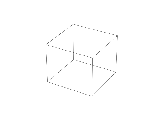
For example, consider the triquadratic hexahedral element and the default cube mesh:

>>> from skfem import *
>>> m = MeshHex()
>>> m
<skfem MeshHex1 object>
  Number of elements: 1
  Number of vertices: 8
  Number of nodes: 8
>>> basis = Basis(m, ElementHex2())
>>> basis
<skfem CellBasis(MeshHex1, ElementHex2) object>
  Number of elements: 1
  Number of DOFs: 27
  Size: 296352 B

(png, hires.png, pdf)

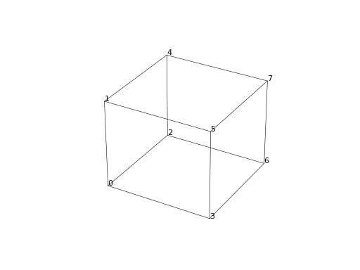
The DOFs corresponding to the nodes (or vertices) of the mesh are

>>> basis.nodal_dofs
array([[0, 1, 2, 3, 4, 5, 6, 7]], dtype=int32)

This means that the first (zeroth) entry in the DOF array corresponds to the first node/vertex in the finite element mesh (see m.p for a list of nodes/vertices).

(png, hires.png, pdf)

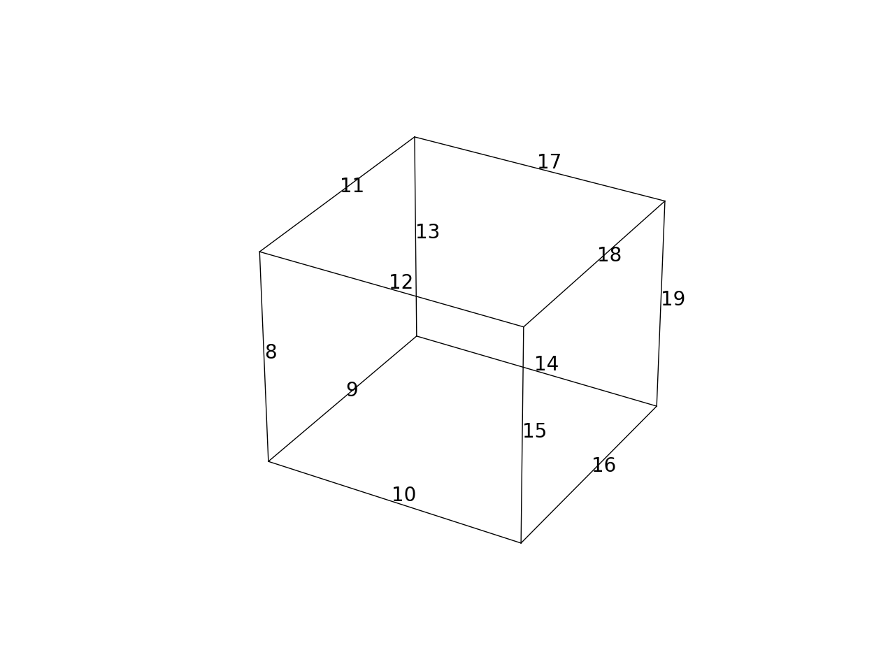
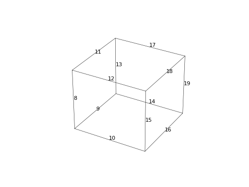
Similarly, the DOFs corresponding to the edges (m.edges for a list of edges) and the facets (m.facets for a list of facets) of the mesh are

>>> basis.edge_dofs
array([[ 8,  9, 10, 11, 12, 13, 14, 15, 16, 17, 18, 19]], dtype=int32)
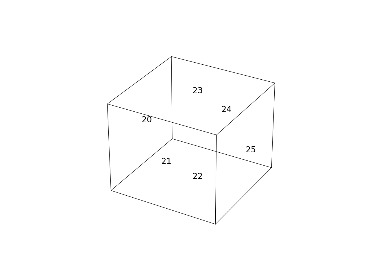
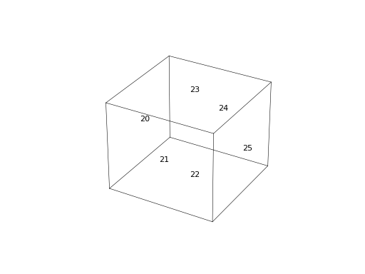
>>> basis.facet_dofs
array([[20, 21, 22, 23, 24, 25]], dtype=int32)

(png, hires.png, pdf)

(png, hires.png, pdf)

All DOFs in nodal_dofs, edge_dofs and facet_dofs are shared between neighbouring elements to preserve continuity. The remaining DOFs are internal to the element and not shared:

>>> basis.interior_dofs
array([[26]], dtype=int32)

Each DOF is associated either with a node (nodal_dofs), a facet (facet_dofs), an edge (edge_dofs), or an element (interior_dofs).