Extended tutorial

Note

This is a tutorial for understanding the classes Mesh and Basis and how they relate to numpy arrays used in skfem to represent finite element functions.

It is extremely helpful when working with skfem to understand the concepts of quadrature points and degrees-of-freedom, and how these concepts relate to symbolic math expressions, Python functions, and real-world data. This all happens in the umbrella concept of a “mesh” and which also has to be reasonably well understood to use skfem. To illustrate how these components fit together, we start with a simple 2D mesh of triangles created directly from skfem.

>>> import matplotlib.pyplot as plt
>>> import numpy as np
>>> import skfem
>>> mesh = skfem.MeshTri()

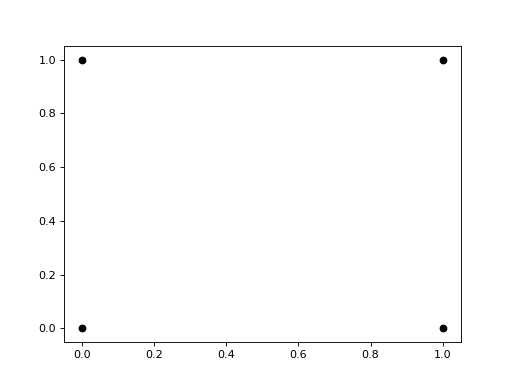
The mesh is represented as two lists of information. The first is a list of points describing where vertexes are and the second is a list of connections between the points to form elements. These connections are the “topology” of the mesh.

>>> mesh.p  # the list of points
array([[0., 1., 0., 1.],
       [0., 0., 1., 1.]])

>>> mesh.t  # the topology
array([[0, 1],
       [1, 2],
       [2, 3]], dtype=int32)

This is easy enough to draw in matplotlib. The first row in the points array contains the x locations of each point and the second row contains the y locations.

plt.plot(mesh.p[0], mesh.p[1], 'ok')

(png, hires.png, pdf)

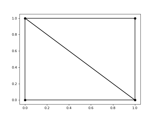
The topology (mesh.t) specifies how these points are connected together to form triangles. Each column specifes the indexes of the points that defined the vertexes of the triangle. We can add these lines to the plot.

plt.plot(mesh.p[0], mesh.p[1], 'ok')
for t in mesh.t.T: # transpose to iterate over columns
    plt.plot(mesh.p[0,[t[0],t[1]]], mesh.p[1,[t[0],t[1]]], 'k')  # from vertex 0 to 1
    plt.plot(mesh.p[0,[t[1],t[2]]], mesh.p[1,[t[1],t[2]]], 'k')  # from vertex 1 to 2
    plt.plot(mesh.p[0,[t[2],t[0]]], mesh.p[1,[t[2],t[0]]], 'k')  # from vertex 2 back to 0

(png, hires.png, pdf)

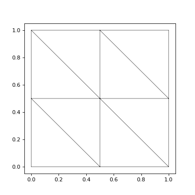
This is the most basic triangulation of the unit square. skfem has utilities to refine this mesh into more and smaller triangles as well as translate it or map it into different coordinates. It also has some basic visualization functions to make drawing the mesh on an matplotlib axis easier.

import skfem.visuals.matplotlib
mesh = skfem.MeshTri().refined(1)
plt.subplots(figsize=(5,5))
skfem.visuals.matplotlib.draw(mesh, ax=plt.gca())  # gca: "get current axis"

(png, hires.png, pdf)

The skfem documentation and code uses several terms when working with meshes of one, two, or three dimensions that are worth clarifying before we proceed. These are cells/elements, facets, edges, and nodes, and are best illustrated with a picture:

The naming conventions used in skfem.

Using this naming convention, facets are always shared between cells/elements and one dimension lower than the mesh. nodes are always at the vertices of the mesh. This picture also illustrates quadrilateral meshes, which are an alternative to triangulations that can be generated by skfem. For the remainder of this discussion, we will work with 2D triangular meshes.

Meshes form a kind of coordinate system to work in, and we construct a set of basis functions in this system by specifying a functional form over one cell/element of the mesh. This discussion will be limited to two kinds of basis functions: ones that are constant over the cell/element and ones that are linear over the cell/element. skfem calls these ElementTriP0 and ElementTriP1, respectively. Note that these two basis sets have different continuity characteristics between cells/elements. Basis functions in ElementTriP0 are discontinuous between cells/elements. Basis functions in ElementTriP1 are continuous between adjacent cells/elements, but their derivatives are not.

We continue this discussion by building a set of basis functions using ElementTriP1 over the once refined triangulation of the unit square discussed above.

>>> basis_p1 = skfem.Basis(mesh, skfem.ElementTriP1())
>>> print(type(basis_p1))
<class 'skfem.assembly.basis.cell_basis.CellBasis'>

What we get back after this call is a Python object of type CellBasis. This is a mostly opaque object that we can use to work with the set of basis functions that span our finite element space. Functions represented in this finite space are (obviously) described by a finite number of parameters, in skfem called the degrees-of-freedom (dofs). In our P1 space that we’ve constructed, this will always be equal to the number of nodes in the mesh. However, this is in general not true, so to get a numpy array of the correct length and initialized to zeros, we will use our basis object.

fe_approximation = basis_p1.zeros()

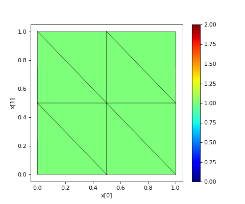
Although this is a simple numpy array, there are not many things we can do with it directly, since out at this level of the code we don’t know anything about what the array index means. Its primary application in our code will be controlling Dirichlet boundary conditions: those locations on the mesh where we already know the value of the solution. We can experiment with this by projecting a constant function of 1 into the finite element space, and then showing how we can manipulate this function using our basis_p1 object and the fe_approximation array. For now, we will also make use of another helper function from skfem to visualize the functions we construct. Later we’ll explore other ways to interrogate and visualize functions we’ve represented in our finite element space.

fe_approximation[:] = 1  # a function that is 1 everywhere; [:] means "all dofs"
plt.subplots(figsize=(6,5))
skfem.visuals.matplotlib.plot(basis_p1, fe_approximation, vmin=0, vmax=2, ax=plt.gca(), colorbar=True)
skfem.visuals.matplotlib.draw(mesh, ax=plt.gca())
plt.xlabel('x[0]'); plt.ylabel('x[1]');

(png, hires.png, pdf)

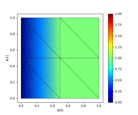
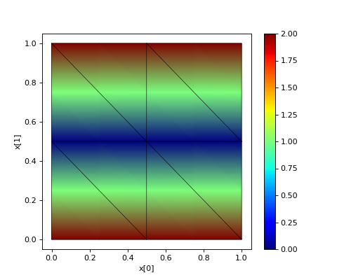
Now, suppose we want to change this function so it is 0 on the left edge. To tell skfem to make the function zero along those vertical line segments on the left edge, we’ll call on a very powerful and flexible feature of our basis object: get_dofs().

We can use this method to make skfem return the indexes to use with fe_approximation in order to specify the value of our function in two ways: along facets and over entire triangles (skfem calls these triangles “cells”/”elements”. In this context, “cell”/”element” is purely geometrical and should not be confused with the “finite element” which includes a concept of polynomial degree.)

def is_on_left_edge(x):
    return x[0] < 0.1
dof_subset_left_edge = basis_p1.get_dofs(facets=is_on_left_edge)
fe_approximation[dof_subset_left_edge] = 0
plt.subplots(figsize=(6,5))
skfem.visuals.matplotlib.plot(basis_p1, fe_approximation, vmin=0, vmax=2, ax=plt.gca(), colorbar=True, shading='gouraud')
skfem.visuals.matplotlib.draw(mesh, ax=plt.gca())
plt.xlabel('x[0]'); plt.ylabel('x[1]');

(png, hires.png, pdf)

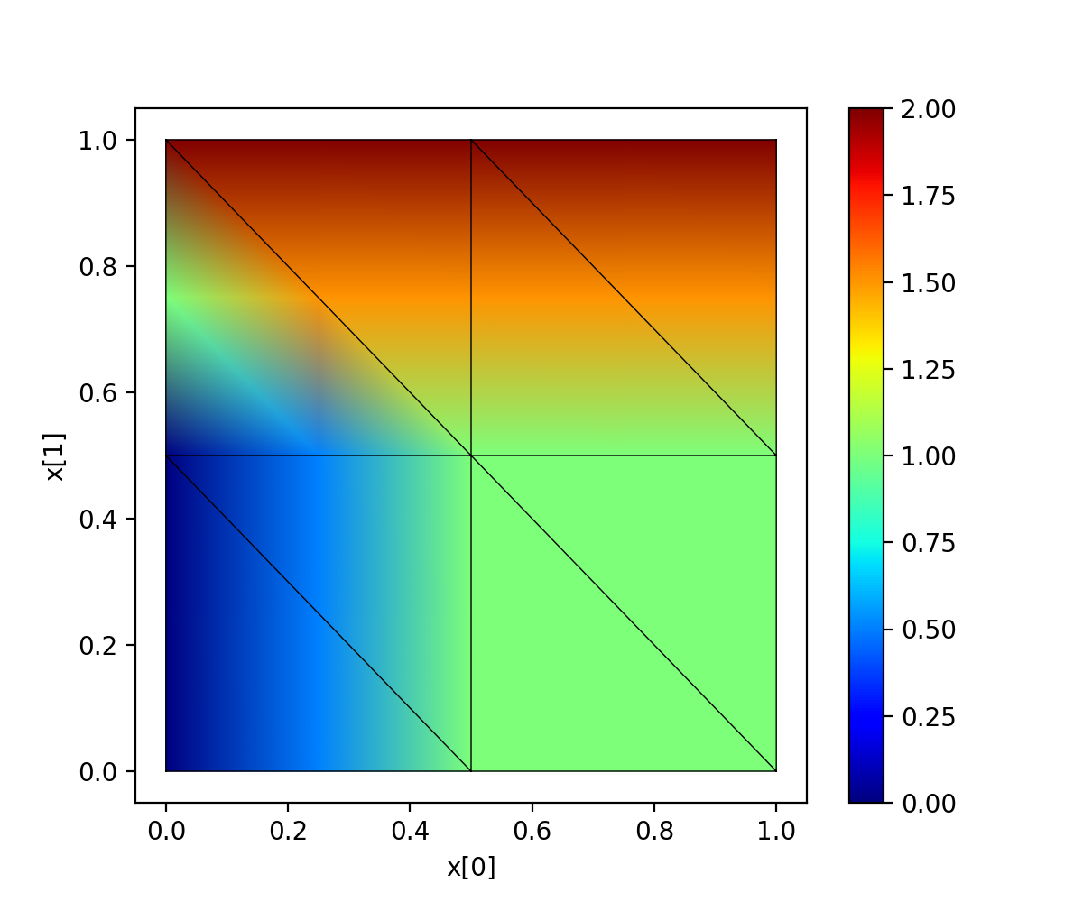
We could make a more complicated function, leaving 0 on that left edge, and going to 2 on the top edge. Here we use a lambda function to make the code more compact. In general though, lambda functions should only be used in trivial circumstances. The verbose naming above is more descriptive and readable.

dof_subset_top_edge = basis_p1.get_dofs(facets=lambda x: x[1] > 0.9)
fe_approximation[dof_subset_top_edge] = 2
plt.subplots(figsize=(6,5))
skfem.visuals.matplotlib.plot(basis_p1, fe_approximation, vmin=0, vmax=2, ax=plt.gca(), colorbar=True, shading='gouraud')
skfem.visuals.matplotlib.draw(mesh, ax=plt.gca())
plt.xlabel('x[0]'); plt.ylabel('x[1]');

(png, hires.png, pdf)

In a directly analogous manner, we can specify values over entire elements instead of just edges.

# reset the function to be 1 everywhere
fe_approximation[:] = 1
dof_subset_bottom_left = basis_p1.get_dofs(elements=lambda x: np.logical_and(x[0]<.3, x[1]<.3))
fe_approximation[dof_subset_bottom_left] = 0
plt.subplots(figsize=(6,5))
skfem.visuals.matplotlib.plot(basis_p1, fe_approximation, vmin=0, vmax=2, ax=plt.gca(), colorbar=True, shading='gouraud')
skfem.visuals.matplotlib.draw(mesh, ax=plt.gca())
plt.xlabel('x[0]'); plt.ylabel('x[1]');

(png, hires.png, pdf)

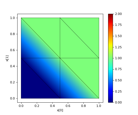
This is exactly correct. The function is 0 everywhere in the bottom left triangle, and goes linearly (because we’re in P1) to 1 outside of this triangle. Note the continuity between triangles, another consequence of using P1 to form our basis set.

To summarize our discussion so far, we’ve seen how to construct a finite element basis set from a mesh and a choice of function over one cell of that mesh, in our case P1 (linear polynomials). And we’ve now seen how to create simple functions in that space by specifying the value of the function everywhere ([:]), along facets (get_dofs(facets=...)) or over elements (get_dofs(elements=...)).

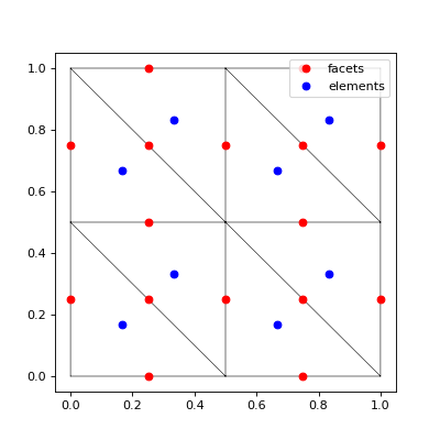
Lets take a closer look at what is happening when we supply a function to get_dofs() by tricking it into plotting the query locations it is using. Note the use of lambda here to supply most of the arguments to our trial function while still leaving x available as an argument for get_dofs().

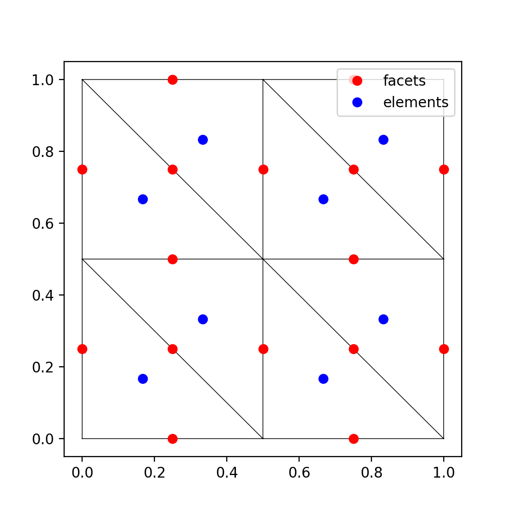
def plot_query_points(x, ax, style, label):
    ax.plot(x[0], x[1], style, label=label)
    return x[0] * 0
plt.subplots(figsize=(5,5))
skfem.visuals.matplotlib.draw(mesh, ax=plt.gca())
basis_p1.get_dofs(facets=lambda x: plot_query_points(x, plt.gca(), 'or', 'facets'))
basis_p1.get_dofs(elements=lambda x: plot_query_points(x, plt.gca(), 'ob', 'elements'))
plt.legend()

(png, hires.png, pdf)

This plot shows the x coordinates supplied to our test function. If we return True for one of these coordinates, then get_dofs() will return the indexes required by fe_approximation to force that element or facet to a specified value.

The extremely important caveat here is that one should never use == when dealing with floating point numbers. Therefore, to find those two red dots on the vertical pair of facets in the center, we should write as follows. (Later we will show more robust and precise ways of labelling facets and elements during mesh construction.)

dof_subset_vertical_centerline = basis_p1.get_dofs(facets=lambda x: np.isclose(x[0], 0.5))
fe_approximation[:] = 2
fe_approximation[dof_subset_vertical_centerline] = 0
plt.subplots(figsize=(6,5))
skfem.visuals.matplotlib.plot(basis_p1, fe_approximation, vmin=0, vmax=2, ax=plt.gca(), colorbar=True, shading='gouraud')
skfem.visuals.matplotlib.draw(mesh, ax=plt.gca())
plt.xlabel('x[0]'); plt.ylabel('x[1]');

(png, hires.png, pdf)

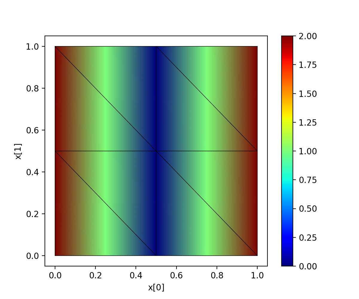
Another way to construct a function in the finite element space is by projection. To demonstrate this, we’ll use f(x) = abs(x[1]-0.5) which would be a horizontal valley running along the line at x[1]=0.5. We’ll use an skfem utility which uses a CellBasis object to project a Python function into the finite element space. The corresponding Python function must accept a single argument of point vectors and return an array of function values at those points.

def f(x):
    return 4 * abs(x[1] - 0.5)
fe_approximation = basis_p1.project(f)
plt.subplots(figsize=(6,5))
skfem.visuals.matplotlib.plot(basis_p1, fe_approximation, vmin=0, vmax=2, ax=plt.gca(), colorbar=True, shading='gouraud')
skfem.visuals.matplotlib.draw(mesh, ax=plt.gca())
plt.xlabel('x[0]'); plt.ylabel('x[1]');

(png, hires.png, pdf)

Compare the similarities between this example and the previous one to see how there may be more than one way to construct the same function in our finite element space. From this point forward, we will refer to this process generically as “projecting into the finite element space” regardless of which of the methods was actually used to generate the projection.

The basis_p1 object and the fe_approximation array that we’ve been working with are abstract representations of our function in the finite element space. Internally, skfem samples this function at a set of locations called “quadrature points”. skfem uses weight sums of these samples to compute the integrals it uses to solve PDEs.

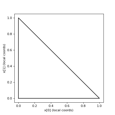
These samples at quadrature points are another way to represent the functions we have projected into finite element space and it is important to understand their relationship with the projections we’ve been constructing. To start this discussion, however, it is important to distinguish between “local” coordinates and “global” coordinates. In this triangulation we’ve been working in, the local, or reference, triangle is within the unit square with vertexes and (0, 0), (1, 0), and (0, 1).

plt.subplots(figsize=(5,5))
plt.plot([0,1,0,0], [0,0,1,0], 'k')
plt.xlabel('x[0] (local coords)'); plt.ylabel('x[1] (local coords)');

(png, hires.png, pdf)

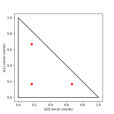
Each of the triangles in our mesh can be individually be transformed into these coordinates, i.e. for the purposes of integration. The quadrature points used are available via the basis object we constructed previously, so we can plot their locations on the reference triangle.

plt.subplots(figsize=(5,5))
plt.plot([0,1,0,0], [0,0,1,0], 'k')
points, weights = basis_p1.quadrature
plt.plot(points[0], points[1], 'or')
plt.xlabel('x[0] (local coords)'); plt.ylabel('x[1] (local coords)');

(png, hires.png, pdf)

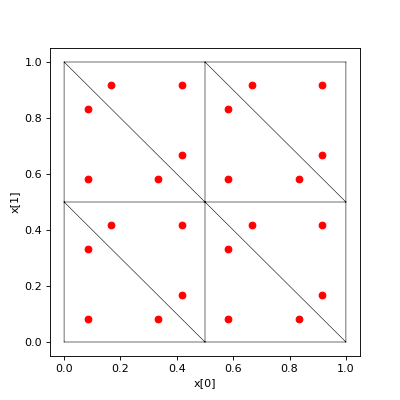
We can get a global visualization of the quadrature points by reverse mapping the local coordinates to each of the triangles in our mesh.

global_points = basis_p1.mapping.F(points)
plt.subplots(figsize=(5,5))
plt.plot(global_points[0], global_points[1], 'or')
skfem.visuals.matplotlib.draw(mesh, ax=plt.gca())
plt.xlabel('x[0]'); plt.ylabel('x[1]');

(png, hires.png, pdf)

The global_points array is organized as (coordinate, element_index, quadrature_index):

>>> global_points.shape  # 2 dimensional, 8 elements, 3 points/element
(2, 8, 3)

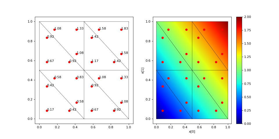
To demonstrate how interpolation works, let’s annotate each of those quadrature points with the values of a (projected) function sampled at those locations. To do this, we’ll use the interpolate method of our basis object on a function projected into finite element space.

def f(x):
    return x[0] + x[1]
fe_approximation = basis_p1.project(f)
interpolation = basis_p1.interpolate(fe_approximation)
global_points = basis_p1.mapping.F(points).reshape(2, -1)
fig, ax = plt.subplots(1, 2, figsize=(12,6))
skfem.visuals.matplotlib.draw(mesh, ax=ax[0])
for value, p in zip(interpolation.value.reshape(-1), global_points.T):
    ax[0].plot(p[0], p[1], 'or')
    ax[0].annotate(f'{value:.2f}', [p[0], p[1]])
skfem.visuals.matplotlib.plot(basis_p1, fe_approximation, vmin=0, vmax=2, ax=ax[1], shading='gouraud', colorbar=True)
skfem.visuals.matplotlib.draw(mesh, ax=ax[1])
ax[1].plot(global_points[0], global_points[1], 'or')
plt.xlabel('x[0]'); plt.ylabel('x[1]');

(png, hires.png, pdf)

The number of quadrature points in an element controls the level of accuracy of the integrations. For low degree polynomial basis functions, one can supply enough quadrature points for exact integration, where the only source of error is the finite machine precision of the computer. Using more quadrature points than necessary does not further improve accuracy and slightly increases computation time, but it can provide a common space to perform computations on functions that were projected into different finite element spaces.

For this reason, it is usually preferred to construct the highest order basis set first (in the present consideration that is P1) and then derive the lower order basis set from it. This will ensure the basis sets share a common set of quadrature points, and that there are enough quadrature points to perform exact integration of the highest order basis set.

basis_p0 = basis_p1.with_element(skfem.ElementTriP0())

The P0 space has functions that are constant over a cell/element in the mesh and consequently discontinuous on the facets between cells/elements. It also has fewer degrees-of-freedom than a P1 basis constructed on the same mesh. Specifically, the P0 basis will have a degree-of-freedom for each cell/element in the mesh.

>>> print(f'{basis_p1.zeros().shape[0]} dofs in P1 == {mesh.p.shape[1]} nodes in the mesh')
>>> print(f'{basis_p0.zeros().shape[0]} dofs in P0 == {mesh.t.shape[1]} elements in the mesh')
9 dofs in P1 == 9 nodes in the mesh
8 dofs in P0 == 8 elements in the mesh

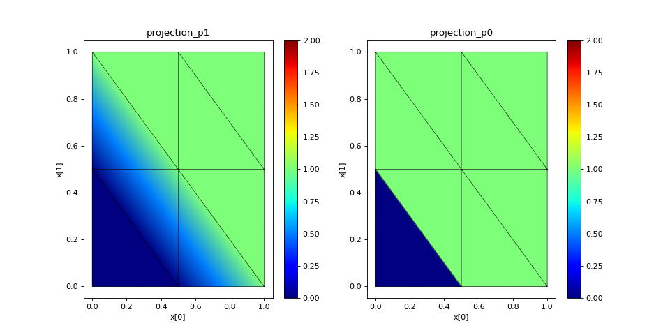
Functions can be projected into the P0 space in the same ways that were used for P1 projection: get_dofs() and project(). As the first example, we will examine get_dofs() and compare it to one of the previous examples we used in P1: the lower left triangle should be 0 and 1 everywhere else in the mesh.

# reset the function to be 1 everywhere
projection_p1 = basis_p1.zeros()
projection_p0 = basis_p0.zeros()
projection_p1[:] = 1
projection_p0[:] = 1

def is_bottom_left(x):
    return np.logical_and(x[0]<.3, x[1]<.3)

p1_bottom_left = basis_p1.get_dofs(elements=is_bottom_left)
p0_bottom_left = basis_p0.get_dofs(elements=is_bottom_left)
projection_p1[p1_bottom_left] = 0
projection_p0[p0_bottom_left] = 0

fig, ax = plt.subplots(1, 2, figsize=(12,6))
skfem.visuals.matplotlib.plot(basis_p1, projection_p1, vmin=0, vmax=2, ax=ax[0], shading='gouraud', colorbar=True)
skfem.visuals.matplotlib.draw(mesh, ax=ax[0])
skfem.visuals.matplotlib.plot(basis_p0, projection_p0, vmin=0, vmax=2, ax=ax[1], shading='gouraud', colorbar=True)
skfem.visuals.matplotlib.draw(mesh, ax=ax[1])
ax[0].set_xlabel('x[0]'); ax[0].set_ylabel('x[1]')
ax[1].set_xlabel('x[0]'); ax[1].set_ylabel('x[1]')
ax[0].set_title('projection_p1'); ax[1].set_title('projection_p0');

(png, hires.png, pdf)

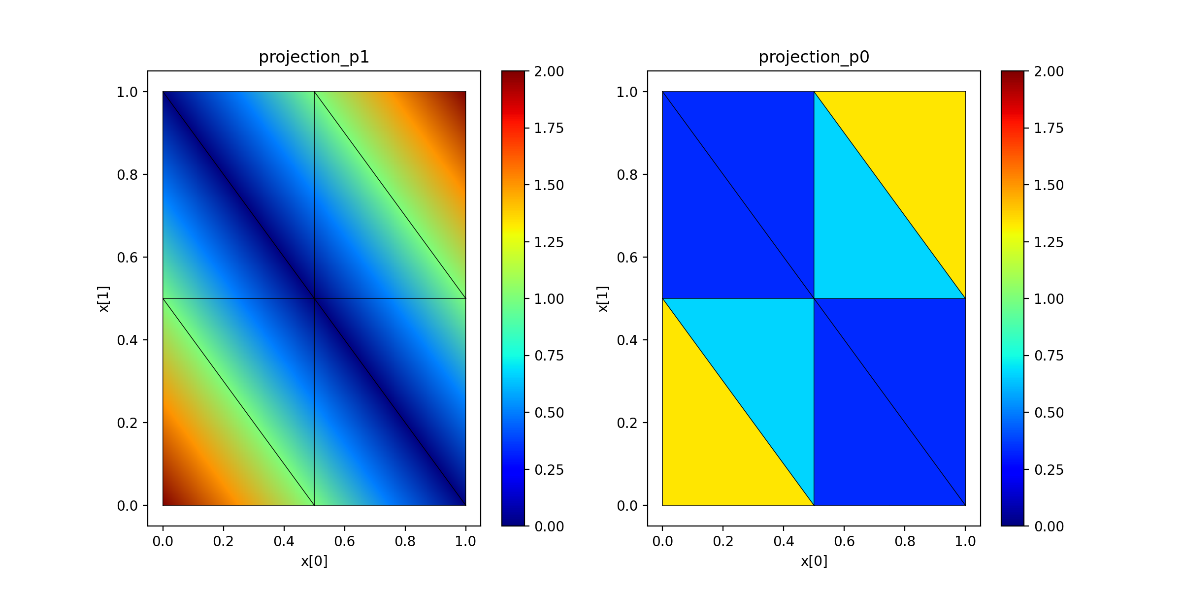
A second example of functions projected into P0 uses project():

def f(x):
    return 2 * abs(x[0] + x[1] - 1)
projection_p1 = basis_p1.project(f)
projection_p0 = basis_p0.project(f)
fig, ax = plt.subplots(1, 2, figsize=(12,6))
skfem.visuals.matplotlib.plot(basis_p1, projection_p1, vmin=0, vmax=2, ax=ax[0], shading='gouraud', colorbar=True)
skfem.visuals.matplotlib.draw(mesh, ax=ax[0])
skfem.visuals.matplotlib.plot(basis_p0, projection_p0, vmin=0, vmax=2, ax=ax[1], shading='gouraud', colorbar=True)
skfem.visuals.matplotlib.draw(mesh, ax=ax[1])
ax[0].set_xlabel('x[0]'); ax[0].set_ylabel('x[1]')
ax[1].set_xlabel('x[0]'); ax[1].set_ylabel('x[1]')
ax[0].set_title('projection_p1'); ax[1].set_title('projection_p0');

(png, hires.png, pdf)

It is critical to realize in both of the previous two examples, the identical “real” function was projected into each of the P1 and P0 spaces, and the plots are showing the closest approximation to the “real” function available in the respective spaces.

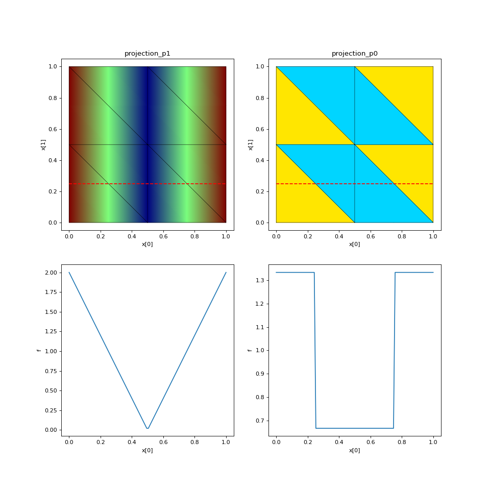
To gain further insight into how well these projections are matching our “real” functions, it would be useful to examine these projections along a line through the space. For this, we can use the probes method on the basis objects we have constructed. Let’s use f(x) = 4 * abs(x[0] - 0.5) to illustrate how this works.

N_query_pts = 100
x1_value = 0.25
query_pts = np.vstack([
    np.linspace(0,1,N_query_pts),  # x[0] coordinate values
    x1_value*np.ones(N_query_pts),  # x[1] coordinate values
])
p1_probes = basis_p1.probes(query_pts)
p0_probes = basis_p0.probes(query_pts)

def f(x):
    return 4 * abs(x[0] - 0.5)

projection_p1 = basis_p1.project(f)
projection_p0 = basis_p0.project(f)

fig, ax = plt.subplots(2, 2, figsize=(12,12))
skfem.visuals.matplotlib.plot(basis_p1, projection_p1, vmin=0, vmax=2, ax=ax[0][0], shading='gouraud')
skfem.visuals.matplotlib.draw(mesh, ax=ax[0][0])
ax[0][0].plot(query_pts[0], query_pts[1], '--r')
skfem.visuals.matplotlib.plot(basis_p0, projection_p0, vmin=0, vmax=2, ax=ax[0][1], shading='gouraud')
skfem.visuals.matplotlib.draw(mesh, ax=ax[0][1])
ax[0][1].plot(query_pts[0], query_pts[1], '--r')
ax[0][0].set_xlabel('x[0]'); ax[0][0].set_ylabel('x[1]')
ax[0][1].set_xlabel('x[0]'); ax[0][1].set_ylabel('x[1]')
ax[0][0].set_title('projection_p1'); ax[0][1].set_title('projection_p0');

ax[1][0].plot(query_pts[0], p1_probes @ projection_p1)
ax[1][0].set_xlabel('x[0]'); ax[1][0].set_ylabel('f')
ax[1][1].plot(query_pts[0], p0_probes @ projection_p0)
ax[1][1].set_xlabel('x[0]'); ax[1][1].set_ylabel('f');

(png, hires.png, pdf)

One more example, using a more refined mesh and a f(x) = sin(2 * pi * x[1]). Note that since we are changing the mesh here, we must also reconstruct the basis objects.

mesh = skfem.MeshTri().refined(5)
basis_p1 = skfem.Basis(mesh, skfem.ElementTriP1())
basis_p0 = basis_p1.with_element(skfem.ElementTriP0())

N_query_pts = 200
x0_value = .5
query_pts = np.vstack([
    x0_value * np.ones(N_query_pts),  # x[0] coordinate values
    np.linspace(0,1,N_query_pts),  # x[1] coordinate values
])
p1_probes = basis_p1.probes(query_pts)
p0_probes = basis_p0.probes(query_pts)

def f(x):
    return np.sin(2 * np.pi * x[1])

projection_p1 = basis_p1.project(f)
projection_p0 = basis_p0.project(f)

fig, ax = plt.subplots(2, 2, figsize=(12,12))
skfem.visuals.matplotlib.plot(basis_p1, projection_p1, vmin=0, vmax=2, ax=ax[0][0], shading='gouraud')
skfem.visuals.matplotlib.draw(mesh, ax=ax[0][0])
ax[0][0].plot(query_pts[0], query_pts[1], '--r')
skfem.visuals.matplotlib.plot(basis_p0, projection_p0, vmin=0, vmax=2, ax=ax[0][1], shading='gouraud')
skfem.visuals.matplotlib.draw(mesh, ax=ax[0][1])
ax[0][1].plot(query_pts[0], query_pts[1], '--r')
ax[0][0].set_xlabel('x[0]'); ax[0][0].set_ylabel('x[1]')
ax[0][1].set_xlabel('x[0]'); ax[0][1].set_ylabel('x[1]')
ax[0][0].set_title('projection_p1'); ax[0][1].set_title('projection_p0');

ax[1][0].plot(query_pts[1], p1_probes @ projection_p1)
ax[1][0].set_xlabel('x[1]'); ax[1][0].set_ylabel('f')
ax[1][1].plot(query_pts[1], p0_probes @ projection_p0)
ax[1][1].set_xlabel('x[1]'); ax[1][1].set_ylabel('f');

(png, hires.png, pdf)