Getting started¶

If you have a supported Python installation on your computer, you can install the package via

pip install scikit-fem[all]

Specifying [all] includes meshio for mesh input/output, and matplotlib for simple visualizations. The minimal dependencies are numpy and scipy. You can also install scikit-fem in Google Colab by executing

!pip install scikit-fem

Step 1: Clarify the problem¶

In this tutorial we solve the Poisson problem

\[\begin{split}\begin{aligned} -\Delta u &= f \quad && \text{in $\Omega$,} \\ u &= 0 \quad && \text{on $\partial \Omega$,} \end{aligned}\end{split}\]

where $\Omega = (0, 1)^2$ is a square domain and $f(x,y)=\sin \pi x \sin \pi y$. The weak formulation reads: find $u \in H^1_0(\Omega)$ satisfying

\[\int_\Omega \nabla u \cdot \nabla v \,\mathrm{d}x = \int_\Omega fv\,\mathrm{d}x \quad \forall v \in H^1_0(\Omega).\]

Note

$H^1_0(\Omega)$ is the space of functions that are zero on the boundary $\partial \Omega$ and have finite energy: the square integral of the first derivative is finite.

Step 2: Express the forms as code¶

Next we write the forms

\[a(u, v) = \int_\Omega \nabla u \cdot \nabla v \,\mathrm{d}x \quad \text{and} \quad L(v) = \int_\Omega f v \,\mathrm{d}x\]

as source code. Each form is written as a function and decorated as follows:

>>> import skfem as fem
>>> from skfem.helpers import dot, grad  # helpers make forms look nice
>>> @fem.BilinearForm
... def a(u, v, _):
...     return dot(grad(u), grad(v))

>>> import numpy as np
>>> @fem.LinearForm
... def L(v, w):
...     x, y = w.x  # global coordinates
...     f = np.sin(np.pi * x) * np.sin(np.pi * y)
...     return f * v

For more information see Anatomy of forms.

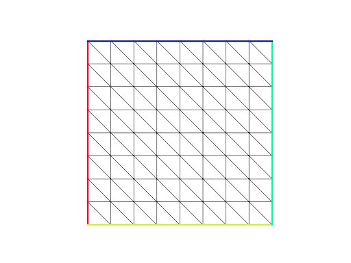
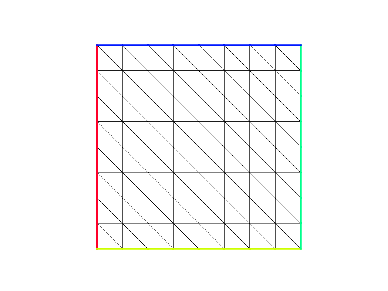
Step 3: Create a mesh¶

The default constructors of Mesh initialize a unit square:

>>> mesh = fem.MeshTri().refined(3)  # refine thrice
>>> mesh
<skfem MeshTri1 object>
  Number of elements: 128
  Number of vertices: 81
  Number of nodes: 81
  Named boundaries [# facets]: left [8], bottom [8], right [8], top [8]

(png, hires.png, pdf)

Step 4: Define a basis¶

The mesh is combined with a finite element to form a global basis. Here we choose the piecewise-linear basis:

>>> Vh = fem.Basis(mesh, fem.ElementTriP1())
>>> Vh
<skfem CellBasis(MeshTri1, ElementTriP1) object>
  Number of elements: 128
  Number of DOFs: 81
  Size: 27648 B

Step 5: Assemble the linear system¶

Now everything is in place for the finite element assembly. The resulting matrix has the type scipy.sparse.csr_matrix and the load vector has the type ndarray.

>>> A = a.assemble(Vh)
>>> l = L.assemble(Vh)
>>> A.shape
(81, 81)
>>> l.shape
(81,)

Step 6: Find boundary DOFs¶

Setting boundary conditions requires finding the degrees-of-freedom (DOFs) on the boundary. Empty call to get_dofs() matches all boundary DOFs.

>>> D = Vh.get_dofs()
>>> D
<skfem DofsView(MeshTri1, ElementTriP1) object>
  Number of nodal DOFs: 32 ['u']

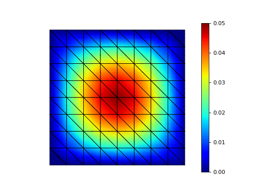
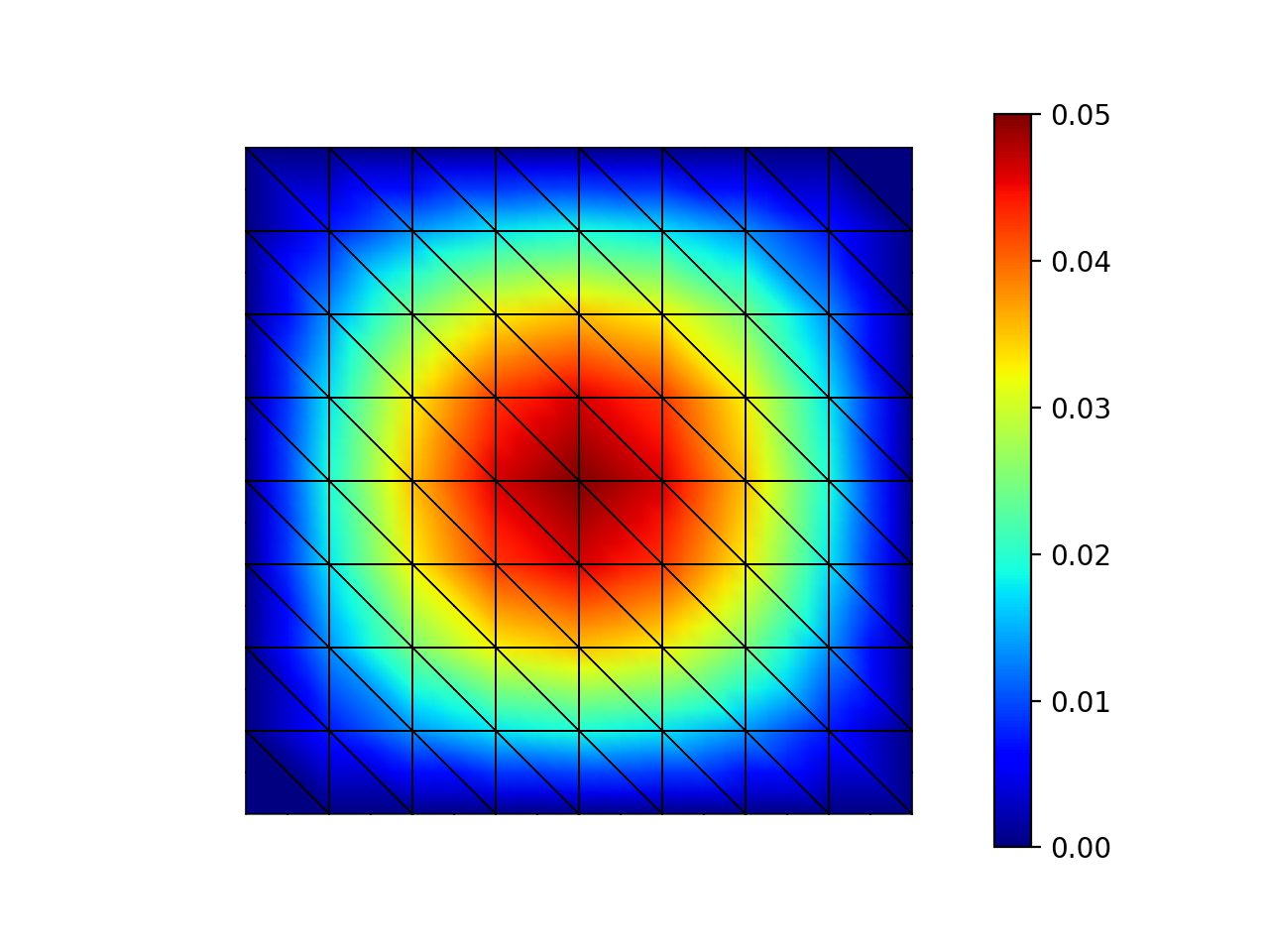
Step 7: Eliminate boundary DOFs and solve¶

The boundary DOFs must be eliminated from the linear system $Ax=l$ to set $u=0$ on the boundary. This can be done using condense(). The output can be passed to solve() which is a simple wrapper to scipy sparse solver:

>>> x = fem.solve(*fem.condense(A, l, D=D))
>>> x.shape
(81,)

(png, hires.png, pdf)

Step 8: Calculate error¶

The exact solution is known to be

\[u(x, y) = \frac{1}{2 \pi^2} \sin \pi x \sin \pi y.\]

Thus, it makes sense to verify that the error is small.

>>> @fem.Functional
... def error(w):
...     x, y = w.x
...     uh = w['uh']
...     u = np.sin(np.pi * x) * np.sin(np.pi * y) / (2. * np.pi ** 2)
...     return (uh - u) ** 2
>>> str(round(error.assemble(Vh, uh=Vh.interpolate(x)), 9))
'1.069e-06'